For resource-poor languages such as Hmong, large datasets of annotated questions are unavailable, which means that producing an automated question classifier is a potentially challenging task. Currently, a dataset containing 411 annotated Hmong questions is publicly available. The challenge here is to produce a question classifier with adequate accuracy using this available dataset.
What we are exploring here is how well certain models perform with an intentionally limited set of data. This will allow us to gain a better understanding about what kinds of model architectures would work best in the long-term for resource-poor languages, which in most cases will never have the kind of robust data that produce SOTA results in more prominent languages.
We will test five different models with our dataset and compare their accuracy:
- Three-layer MLP using word embeddings
- Double BiLSTM
- Ordered Bidirectional GRU with a Simple RNN
- Three-layer MLP using a CountVectorizer
- Three-layer MLP using a bigram CountVectorizer and weights regularization
Let’s begin by importing the modules we need to preprocess the data.
import os
import sys
import re

import numpy as np
from gensim.models import KeyedVectors
from keras.preprocessing.text import Tokenizer
from keras.preprocessing.sequence import pad_sequences
from keras.utils.np_utils import to_categorical
from sklearn.model_selection import train_test_split

pos_tag_interface_path = os.path.expanduser(os.path.join('~',
                                                         'python_workspace',
                                                         'medical_corpus_scripting',
                                                         'pos_tagger_interface'))
sys.path.append(pos_tag_interface_path)
from POS_Tagger import HmongPOSTagger
Next, we load the KeyedVectors based on the models that are part of the Hmong Medical Corpus (HMC):
- Subword embeddings based on the annotated HMC data (to handle syllable-based spacing in Hmong)
- POS tag embeddings based on the annotated HMC data
- Token embeddings based on the SCH (soc.culture.hmong) Corpus
subword_embeddings = KeyedVectors.load('subword_model.h5', mmap='r')
tag_embeddings = KeyedVectors.load('tag_alone_model.h5', mmap='r')
token_embeddings = KeyedVectors.load('word2vec_Hmong_SCH.model', mmap='r')
Next, we load the annotated question dataset from the relevant file.
def load_question_data(filename):
    f = open(filename, 'r')
    data = [w.strip().split(' | ') for w in f.readlines() if '???' not in w and '<' not in w]
    f.close()
    print(len(data))
    return data
data = load_question_data('question_type_training_set_2.txt')
The dataset contains an uneven distribution of examples: it reflects the kinds of questions for which annotated data are available. This means we need to produce a smaller dataset with an even amount of examples for each category.
Ensuring this, however, means that our dataset of 411 examples will shrink down to 135, given 15 examples for each category.
from collections import Counter

c = Counter(w[1] for w in data)

sorted_data = sorted(list(c.items()), key=lambda item: item[1], reverse=True)
print(sorted_data)

first_filtered_data = [w for w in data if c[w[1]] >= 15]
#filtered_data = [w for w in data if c[w[1]] > 2]

total_count = {w[0]: 0 for w in sorted_data}

filtered_data = []
for item in first_filtered_data:
    if total_count[item[1]] < 15:
        filtered_data.append(item)
        total_count[item[1]] += 1

print(len(filtered_data))

print(total_count.items())
For the next step, we split the data into questions and labels using zip.
questions, labels = zip(*filtered_data)
Now, we load the Hmong POS tagger and tag the words that make up the questions. This will produce tags of the sequence subword-POS, as in B-NN for the first syllable of a word, and the unit in question is a noun.
def tag_question_data(questions):
    tagger = HmongPOSTagger()
    tokenized_questions = [re.sub('([\?,;])', ' \g<1>', q).split(' ') for q in questions]
    return tokenized_questions, tagger.tag_words(tokenized_questions)
tokenized_questions, tags = tag_question_data(questions)
Here, we split the subword tags and the POS tags, placing them in separate sentence sets.
def split_subword_pos_tags(tags):
    """This function takes tags of type B-NN (subword-POS)
    and produces separate lists for subword tags and POS tags"""
    subword_tags = []
    pos_tags = []
    for sent in tags:
        subword_sent = []
        pos_sent = []
        for word in sent:
            if word == '-PAD-': # unknown word that needs reassignment
                subword = 'B'
                pos = 'FW'
            else:
                subword, pos = word.split('-')
            subword_sent.append(subword)
            pos_sent.append(pos)
        subword_tags.append(subword_sent)
        pos_tags.append(pos_sent)
    return subword_tags, pos_tags
subword_tags, pos_tags = split_subword_pos_tags(tags)
The next step converts the words, tags, and labels to integers using keras.preprocessing.text.Tokenizer and sets the values for -PAD- and -OUT-.
# notes: keras.preprocessing.text.one_hot, text_to_word_sequence
# special pad values are used because Keras Tokenizer does not permit 0 as a value
tokenizer = Tokenizer()
tokenizer.fit_on_texts(tokenized_questions)
# automatically converts words to sequences of numbers
sequences = tokenizer.texts_to_sequences(tokenized_questions)
word_pad_value = max(tokenizer.word_index.values()) + 1
word_out_value = word_pad_value + 1

pos_tag_tokenizer = Tokenizer()
pos_tag_tokenizer.fit_on_texts(pos_tags)
pos_sequences = pos_tag_tokenizer.texts_to_sequences(pos_tags)
pos_pad_value = max(pos_tag_tokenizer.word_index.values()) + 1
pos_out_value = pos_pad_value + 1

subword_tag_tokenizer = Tokenizer()
subword_tag_tokenizer.fit_on_texts(subword_tags)
subword_sequences = subword_tag_tokenizer.texts_to_sequences(subword_tags)
subword_pad_value = max(subword_tag_tokenizer.word_index.values()) + 1
subword_out_value = subword_pad_value + 1

# can use label_tokenizer.sequences_to_texts once done
label_tokenizer = Tokenizer()
label_tokenizer.fit_on_texts(labels)
label_sequences = [l[0] for l in label_tokenizer.texts_to_sequences(labels)]
Now, we set the maximum length of the sentences, define the variable word_index for use later, and then pad the input sequences.
MAX_LENGTH = max(len(s) for s in sequences)

word_index = tokenizer.word_index

padded_sequences = pad_sequences(sequences,
                                 maxlen=MAX_LENGTH,
                                 padding='post',
                                 value=word_pad_value)
padded_pos_sequences = pad_sequences(pos_sequences,
                                     maxlen=MAX_LENGTH,
                                     padding='post',
                                     value=pos_pad_value)
padded_subword_sequences = pad_sequences(subword_sequences,
                                         maxlen=MAX_LENGTH,
                                         padding='post',
                                         value=subword_pad_value)
Next, before we split the data into training and test sets, we must first convert the input sentences using CountVectorizer. This ensures that the models using the CountVectorizer data use the same sentences as the other models to ensure we can compare them. The first step in doing this is to produce string sentences that contain the original string of the word, the subword position tag, and the POS tag. Here, I combine all three into individual words processed as single units, as intuitively this will treat mobBNN (that is, the noun mob ‘sickness’ at the beginning of a word as B-NN) as a different word from mobBVV (the verb mob ‘be sick’ at the beginning of a word as B-VV).
from sklearn.feature_extraction.text import CountVectorizer

def join_data(tokenized_questions, subword_tags, pos_tags):
    joined_data = []
    for i, q in enumerate(tokenized_questions):
        joined_sent = []
        for j, word in enumerate(q):
            joined_sent.append(''.join([word, subword_tags[i][j], pos_tags[i][j]]))
        joined_data.append(' '.join(joined_sent))

    print(joined_data[:2])
    return joined_data
Next, we create a CountVectorizer object for unigrams and create vectors for each sentence.
#CountVectorizer needs sentences made of strings.
joined_data = join_data(tokenized_questions, subword_tags, pos_tags)

vectorizer = CountVectorizer()
vectorizer.fit(joined_data)
vectors = np.array([v.toarray()[0] for v in vectorizer.transform(joined_data)])
Now, we create a CountVectorizer object for bigrams.
pure_vectorizer_bigrams = CountVectorizer(ngram_range=(2,2))
pure_vectorizer_bigrams.fit(joined_data)
pure_bigram_vectors = np.array([v.toarray()[0] for v in pure_vectorizer_bigrams.transform(joined_data)])
Once all the input preprocessing is complete, we can split the dataset into training and test sets. We have several different kinds of data as input: the word token sequences, vector sequences representing both unigrams and bigrams, the POS tag sequences, and the subword position tag sequences, along with the output question label sequences. Each of these are split into training and test sets, where all of the training sets contain the same sentences in the same order, as do the test sets.
labels_matrix = to_categorical(np.asarray(label_sequences))

TEST_SIZE = 0.2
VALIDATION_SIZE = 0.2

(X_train,
 X_test,
 X_vector_train,
 X_vector_test,
 X_bigram_vector_train,
 X_bigram_vector_test,
 X_pos_train,
 X_pos_test,
 X_subword_train,
 X_subword_test,
 y_train,
 y_test) = train_test_split(padded_sequences,
                                   vectors,
                                   pure_bigram_vectors,
                                   padded_pos_sequences,
                                   padded_subword_sequences,
                                   label_sequences,
                                   test_size=TEST_SIZE)

word_set = set(word_value for sent in X_train for word_value in sent)
pos_set = set(pos_value for sent in X_pos_train for pos_value in sent)
subword_set = set(subword_value for sent in X_subword_train for subword_value in sent)
Once this is complete, we define a function that will create embedding matrices for each input set that requires it for three of the models we will consider below.
def create_embeddings_matrix(input_set, index_dict, word2vec_source_object, convert_caps=False):
    '''Creates an embedding matrix from preexisting Word2Vec model for use in the Keras Embedding layer
    @param input_set: the set object containing all unique X entries in X_train as numeral values
    @param index_dict: the Tokenizer.word_index dict object containing numerical conversions
    @param word2vec_source_object: the KeyedVectors object containing the vector values for embedding'''
    # $PAD and $OUT remain zeros; they are max(index_dict.values()) + 1 and + 2, respectively
    pad_out_tags_length = 2
    embedding_matrix = np.zeros((max(index_dict.values()) + pad_out_tags_length + 1,
                                 word2vec_source_object.vector_size))
    for token, numeral in index_dict.items():
        if numeral in input_set:
            try:
                if convert_caps == True:
                    word2vec_token_value = token.upper()
                else:
                    word2vec_token_value = token
                embedding_vector = word2vec_source_object.wv[word2vec_token_value]
            except KeyError:
                embedding_vector = None
            if embedding_vector is not None:
                embedding_matrix[numeral] = embedding_vector
    return embedding_matrix
Now, we use the new function to create the matrices for the word inputs, the POS tag inputs, and the subword position tag inputs.
words_embedding_matrix = create_embeddings_matrix(word_set,
                                                  tokenizer.word_index,
                                                  token_embeddings)
pos_embedding_matrix = create_embeddings_matrix(pos_set,
                                                pos_tag_tokenizer.word_index,
                                                tag_embeddings,
                                                True)
subword_embedding_matrix = create_embeddings_matrix(subword_set,
                                                    subword_tag_tokenizer.word_index,
                                                    subword_embeddings,
                                                    True)
Here, we create another function to produce input matrices from the embedding matrices we just created.
def produce_input_matrix(sequences, embedding_matrix):
    output_sequences = []
    for sent in sequences:
        output_sent = []
        for word in sent:
            output_sent.append(embedding_matrix[word])
        output_sequences.append(output_sent)
    return output_sequences
Now, we produce sequence matrices using the function we just created. These will be the input sets for the first three models we’ll consider.
X_train_sequence_matrix = produce_input_matrix(X_train,
                                               words_embedding_matrix)
X_test_sequence_matrix = produce_input_matrix(X_test,
                                              words_embedding_matrix)
X_pos_train_sequence_matrix = produce_input_matrix(X_pos_train,
                                                   pos_embedding_matrix)
X_pos_test_sequence_matrix = produce_input_matrix(X_pos_test,
                                                  pos_embedding_matrix)
X_subword_train_sequence_matrix = produce_input_matrix(X_subword_train,
                                                       subword_embedding_matrix)
X_subword_test_sequence_matrix = produce_input_matrix(X_subword_test,
                                                      subword_embedding_matrix)
Now, we define how large our output vectors should be by defining y_classes on the basis of the total number of categories found among the question labels in our dataset. Then, we convert our y_train and y_test sets to one-hot vectors.
y_classes = max(label_tokenizer.word_index.values()) + 1
y_train = to_categorical(y_train, num_classes=y_classes)
y_test = to_categorical(y_test, num_classes=y_classes)
Next, we import the necessary libraries from Keras to build the models.
from keras.models import Model
from keras.layers import Input, Embedding, Activation, Flatten, Add
from keras.layers import Dense, LSTM, Bidirectional, GRU, SimpleRNN
from keras.callbacks import EarlyStopping
from keras.regularizers import l2
Next, we create a function that will provide plots of the loss and accuracy results.
from matplotlib import pyplot as plt

%matplotlib inline

def plot_metrics(history_obj):
    plt.plot(history_obj.history['loss'], label='Training loss')
    plt.plot(history_obj.history['val_loss'], label='Validation loss')
    plt.legend(loc="upper left")
    plt.show()

    plt.plot(history_obj.history['accuracy'], label='Training accuracy')
    plt.plot(history_obj.history['val_accuracy'], label='Validation accuracy')
    plt.legend(loc="upper left")
    plt.show()
Next, we create a function that can train and test each model.
def run_model(model, countvectorizer=False, bigrams=False, validation=VALIDATION_SIZE):
    if countvectorizer:
        if bigrams:
            model_history = model.fit(np.array(X_bigram_vector_train),
                                      y_train,
                                      batch_size=4,
                                      epochs=50,
                                      validation_split=validation)
            plot_metrics(model_history)
            scores = model.evaluate(np.array(X_bigram_vector_test), y_test)
        else:
            model_history = model.fit(np.array(X_vector_train),
                                      y_train,
                                      batch_size=4,
                                      epochs=50,
                                      validation_split=validation)
            plot_metrics(model_history)
            scores = model.evaluate(np.array(X_vector_test), y_test)
    else:
        model_history = model.fit([X_train_sequence_matrix,
                                   X_pos_train_sequence_matrix,
                                   X_subword_train_sequence_matrix],
                                  y_train,
                                  batch_size=4,
                                  epochs=50,
                                  validation_split=validation)
        plot_metrics(model_history)
        scores = model.evaluate([X_test_sequence_matrix,
                                 X_pos_test_sequence_matrix,
                                 X_subword_test_sequence_matrix],
                                y_test)
    print("Training set accuracy: {result:.2f} percent".format(result= \
                                                               model_history.history['accuracy'][-1]*100))
    if validation > 0.0:
        print("Validation set accuracy: {result:.2f} percent".format(result= \
                                                                 model_history.history['val_accuracy'][-1]*100))
    print("Accuracy: {result:.2f} percent".format(result=(scores[1]*100)))
At this point, we are ready to build and test the models. Our first model is a multilayer perceptron (MLP). This network will have three Dense layers: two hidden layers using a rectified linear unit (ReLU) activation and one output layer using a softmax activation. We also use a Flatten layer between the second hidden layer and the output layer, as our input is sentences made up of words and our output is a single label. That is, each question as input is two-dimensional, while each label as output is one-dimensional, meaning that we need to reduce the dimensionality—exactly what Flatten does.
# Ordered MLP
word_input = Input(shape=(MAX_LENGTH, 150))
pos_input = Input(shape=(MAX_LENGTH, 150))
subword_input = Input(shape=(MAX_LENGTH, 150))
addition_layer = Add()([word_input, pos_input, subword_input])
dense_1 = Dense(256, activation='relu')(addition_layer)
dense_2 = Dense(256, activation='relu')(dense_1)
flatten_layer = Flatten()(dense_2)
dense_3 = Dense(y_classes, activation='softmax')(flatten_layer)

model = Model(inputs=[word_input, pos_input, subword_input], outputs=dense_3)
model.compile(optimizer='adam',
              loss='categorical_crossentropy',
              metrics=['accuracy'])

print(model.summary())
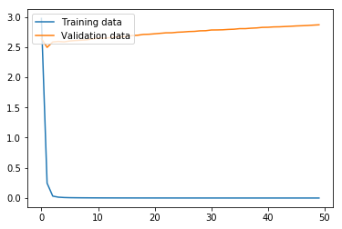
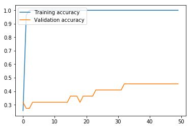
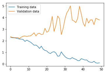
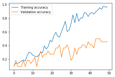
Now we run the MLP model using the function we defined above. As we can see from the graphs, the model effectively converged after only two iterations in regard to the loss, but, interestingly, the validation accuracy continued to increase even as the validation loss slowly increased. In any case, this MLP model produced an accuracy of only 18.52% on the test data, where the variance produced by the limited number of training data proved too problematic for the MLP with the hyperparameters chosen.
run_model(model)
Our second model is a BiLSTM model, which contains two Bidirectional LSTM (Long Short-Term Memory) hidden layers and a Dense layer with a softmax activation as output.
word_bilstm2_input = Input(shape=(MAX_LENGTH, 150))
pos_bilstm2_input = Input(shape=(MAX_LENGTH, 150))
subword_bilstm2_input = Input(shape=(MAX_LENGTH, 150))
addition_bilstm2_layer = Add()([word_bilstm2_input, pos_bilstm2_input, subword_bilstm2_input])
bilstm2_layer = Bidirectional(LSTM(256, return_sequences=True))(addition_bilstm2_layer)
bilstm2_layer_2 = Bidirectional(LSTM(256))(bilstm2_layer)
final_bilstm2_layer = Dense(y_classes, activation='softmax')(bilstm2_layer_2)

model_bilstm2 = Model(inputs=[word_bilstm2_input,
                              pos_bilstm2_input,
                              subword_bilstm2_input],
                      outputs=final_bilstm2_layer)
model_bilstm2.compile(loss='categorical_crossentropy',
                      optimizer='adam',
                      metrics=['accuracy'])

print(model_bilstm2.summary())
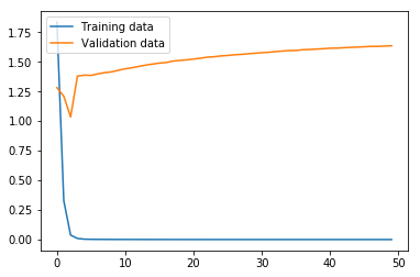
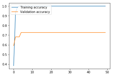
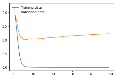
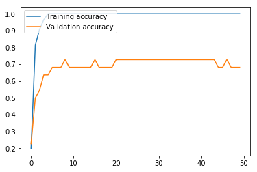
Here, we run the BiLSTM. The results are markedly higher than with our MLP, which is unsurprising, given that the BiLSTM architecture is more appropriate than MLP for ordered sentence data. While our validation loss got progressively worse after only three iterations, the validation accuracy continued to improve until the fifth iteration, and leveled off. The validation accuracy at 72.73% means that this model still struggles with high variance, but the accuracy on the test set at 88.89% means that this model looks promising if the variance is adequately addressed.
run_model(model_bilstm2)
Our third model is a Bidirectional GRU (gated recurrent unit) with a simple RNN (recursive neural network) layer and Dense layer with a softmax activation as output.
# Bidirectional GRU with simple RNN
word_bigru_input = Input(shape=(MAX_LENGTH, 150))
pos_bigru_input = Input(shape=(MAX_LENGTH, 150))
subword_bigru_input = Input(shape=(MAX_LENGTH, 150))
addition_bigru_layer = Add()([word_bigru_input, pos_bigru_input, subword_bigru_input])
bigru_layer = Bidirectional(GRU(256, return_sequences=True))(addition_bigru_layer)
rnn_bigru_layer = SimpleRNN(256, activation='relu')(bigru_layer)
dense_bigru_layer = Dense(y_classes, activation='softmax')(rnn_bigru_layer)

model_bigru = Model(inputs=[word_bigru_input, pos_bigru_input, subword_bigru_input], outputs=dense_bigru_layer)
model_bigru.compile(loss='categorical_crossentropy', optimizer='adam', metrics=['accuracy'])

print(model_bigru.summary())
Now we run the BiGRU. The results suggest that the training loss has not yet converged, which, taken with the training accuracy at 96.51%, would mean the model should be run for more iterations. However, the validation loss and accuracy suggest that the training set and validation sets give quite divergent results. Furthermore, the test set accuracy at 37.04% means the variance adversely affects this model architecture as severely as with the MLP.
run_model(model_bigru)
Next, we try CountVectorizer data with a three-layer MLP.
# CountVectorizer with MLP
bag_word_input = Input(shape=(len(vectors[0]),))
bag_dense_1 = Dense(256, activation='relu')(bag_word_input)
bag_dense_2 = Dense(256, activation='relu')(bag_dense_1)
bag_dense_3 = Dense(y_classes, activation='softmax')(bag_dense_2)
model_cv = Model(inputs=bag_word_input, outputs=bag_dense_3)
model_cv.compile(optimizer='adam', loss='categorical_crossentropy', metrics=['accuracy'])

print(model_cv.summary())
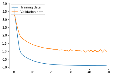
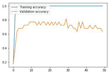
Next, we run the model. This MLP model using CountVectorizer data performs much better than the MLP using word embeddings above. The validation set loss effectively reaches bottom at the seventh iteration, and reaches its maximum accuracy of 72.73% at around iteration 21, meaning that 50 iterations is unnecessary, and in fact slightly hurts the results. Nevertheless, like the other models, this model struggles with variance produced by the small data size, given a final test accuracy of 74.07% versus a training set accuracy of 100.00%.
run_model(model_cv, countvectorizer=True)
Our fifth and final model is a MLP using Bigram CountVectorizer data as input and L2 regularization to prevent early convergence.
# Bigram CountVectorizer with MLP and regularization
bireg_word_input = Input(shape=(len(pure_bigram_vectors[0]),))
bireg_dense_1 = Dense(256, activation='relu', kernel_regularizer=l2(l=0.003))(bireg_word_input)
bireg_dense_2 = Dense(256, activation='relu', kernel_regularizer=l2(l=0.003))(bireg_dense_1)
bireg_dense_3 = Dense(y_classes, activation='softmax')(bireg_dense_2)
model_bireg = Model(inputs=bireg_word_input, outputs=bireg_dense_3)
model_bireg.compile(optimizer='adam', loss='categorical_crossentropy', metrics=['accuracy'])

print(model_bireg.summary())
Again here, we run the model. With Bigram CountVectorizer data and L2 regularization, the model still struggles: the validation accuracy oscillates wildly and declines the longer the model is trained. In the end, a validation set accuracy of 63.64% and a test set accuracy of 85.19% means that L2 regularization did not succeed in handling the variance issue in this case. However, the test set accuracy of 85.19% suggests that with other approaches to handle the variance, this model architecture could prove quite fruitful.
run_model(model_bireg, countvectorizer=True, bigrams=True, validation=0.2)
Conclusion
The results of the five models are shown in the table below.
| Model type |
Input data type | Training Accuracy |
Validation Accuracy |
Test Accuracy |
|---|---|---|---|---|
| MLP | Word embedding | 100.00% | 45.45% | 18.52% |
| BiLSTM | Word embedding | 100.00% | 72.73% | 88.89% |
| BiGRU/ RNN |
Word embedding | 96.51% | 45.45% | 37.04% |
| MLP | CountVectorizer unigram vectors |
100.00% | 68.18% | 74.07% |
| MLP | CountVectorizer bigram vectors |
100.00% | 63.64% | 85.19% |
The results show that BiLSTM is the best architecture for the current problem. The small size of the dataset produced a relatively high degree of variance for all model types, which is naturally expected.
To improve accuracy, that is, to reduce variance in this case, more data combined with the BiLSTM model is the best way to proceed. Given the resource-poor nature of the Hmong language, a set of 30-50 additional examples targeting areas of ambiguity between class types (i.e., question words such as li cas ‘what, why, how’) would be a realistic solution to achieve >90% accuracy.
